The Amazing story of Random Forests!
 Machine Learning Everywhere
Big Data, Machine Learning, Deep Learning, Neural nets, do these words sound familiar? Like you’ve heard them before.
What did the person or place from which you heard these from, tell you about, what they were? If at all they make sense to you or you’re in a state of mind that would make you take a shot at them, here’s how you should try looking at them!
Machine Learning and mathematics always go hand in hand. There's a notion that the newer generation likes to rename the older subjects to make them fancy. If you have heard of the evolution of operations research, this naming and fanciness would make sense.
There are several mathematical analysis methods that are still used in solving many current day problems such as the application of regression, stochastic gradient descent, support vector machines under the name of machine learning.
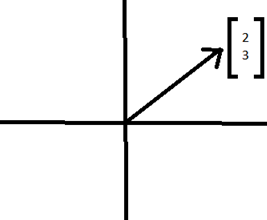
Can they be called machine learning applications? Try and find out.! To be able to solve a problem using machine learning, one must first define the problem in simple parameters/words perse the real physical quantities of the data and the process though which the data is collected. We learnt that the physical property of a phenomenon, a body or a substance that can be observed or quantified by measurement during a scientific study can be termed to be a _Physical Quantity_, generally expressed in terms of numeric values followed by a unit that corresponds to the kind of measurement/subject of study. The broad and widely known classification of them is into physical quantities of the scalars and vectors. Scalars as we know are physical quantities which contain magnitude but no direction. Where as the Vectors are the ones that have both magnitude and direction. ie., a vector is defined by its length and the direction it points to. The vectors that move in a flat plane are two dimensional where as the one's in space may be termed to be three dimensional.In another perspective a vector may be a list of numbers that describes a set of characteristics of a given real world object ie., make the data into a parameterized equation. Vectors can simply be represented by an arrow. The tail of the vector represents the root/ origin where as the head i.e., the arrow head represents the direction in which it is pointing.
 Paint yo!
Consider the vector shown in the figure beside, the numbers in the square braces give the instructions for how to get from the tail of the vector to the head. The first number 2, represents the distance in x direction and the second number 3, represents the distance in y direction.
Every such pair of numbers gives information about only one vector. In a three-dimensional plane we tend to consider an extra dimension z which results in an ordered triplet instead of a pair of numbers, that tells how far to move parallel to the x, y and z axes. Every triplet represents one unique vector in space and vice-versa. Operations such as vector addition, vector product can be performed over the vectors.
 Said what!??
What if we run out of the dimensions we know!
The answer lies right here, matrices and Tensors.
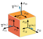
Tensors are physical quantities that are typically of several orders. Scalars are the first of them under the name zeroth order tensors. Vectors on the higher end, that possess a direction along with magnitude fall into the first order tensors symbolized by an arrow in any given geometric plane. Second order tensors are a higher dimensional vectors ie., the vectors that contain information of more than two directions.
What do we do with the tensors/vectors now? Try and observe. Analyse as they call it! But wait, we know something that we all did in our engineering drawing course.
 Tensor
Projection can be understood as a mapping or correspondence between the points of a figure and a surface per se a line isn't it? In plane projections a series of points on one plane are projected onto a second plane by choosing any point as a focus or origin and constructing lines from the chosen origin onto the second plane such that the lines pass through the first plane.
How does drawing projections help me comprehend my data?
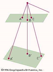 An example of a projection
These kind of projections are dependent on ones' perspective and hence an infinite number of them can be drawn.
Common examples of projections are the shadows that are cast by opaque objects and motion pictures on screen.
This method of constructing projections in different perspectives can be applied to obtain different perspectives of data whilst analysis. It helps us draw conclusions about various aspects of data and construct rules for classification (if any classes are present) or regression.
An example of a projection
These kind of projections are dependent on ones' perspective and hence an infinite number of them can be drawn.
Common examples of projections are the shadows that are cast by opaque objects and motion pictures on screen.
This method of constructing projections in different perspectives can be applied to obtain different perspectives of data whilst analysis. It helps us draw conclusions about various aspects of data and construct rules for classification (if any classes are present) or regression.
Regression/ Regression Analysis is a statistical process for estimating relationships among variables. We all did a linear algebra course where in we used to have equations with x and y equating to a constant. Given n equations finding N unknowns wasn't it simple?
 Regression??? What?
That is the simplest of the examples for regression. What we do in regression is, we look at data from the past, ie., in this case the equations we already have in hand and apply mathematical logic to formulate an equation that gives us an answer. That equation in mathematics world is called as the regression equation(try reading more on this to get a deeper idea). A mathematician would call the plane given by that equation to be a hyperplane or the one that gives him an answer. Regression in data science is a process that helps us understand how the typical value of the dependent variable i.e., a parameter of choice from the data changes, is related when any one of the other independent variables are varied and all others are kept fixed in given dataset.
Regression??? What?
That is the simplest of the examples for regression. What we do in regression is, we look at data from the past, ie., in this case the equations we already have in hand and apply mathematical logic to formulate an equation that gives us an answer. That equation in mathematics world is called as the regression equation(try reading more on this to get a deeper idea). A mathematician would call the plane given by that equation to be a hyperplane or the one that gives him an answer. Regression in data science is a process that helps us understand how the typical value of the dependent variable i.e., a parameter of choice from the data changes, is related when any one of the other independent variables are varied and all others are kept fixed in given dataset.
Regression is commonly used to expect the dependent variable from independent variables on a conditional basis. By doing so we end up estimating the average value of dependent value. Inferences of causal (dependency) relationships between the known quantities and unknown quantity can be made.Sometimes the relations thus established by the regression analysis of data can lead to false results i.e., the correlation may be lesser than what is expected.
</p>
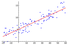 Sample Regression
Random data points and their linear regressionIt is also to be understood that the performance of regression analysis in practise depends upon the form of the data generating process and how it relates to the regression approach is being used in that scenario.
Many a times, since the original process of data generation is not known, we make assumptions about the process generating the data.
I'm involved into a research where the assumption is that the data we generate is an outcome of, collective effect of several random processes, which is ultimately a Gaussian Process.
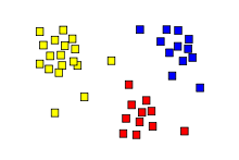 cluster
This assumption(s) is(are) testable if enough amount of data is available, which in our case is abundant.
Now that we have data? What do we do with it? Go feed it to the machine? Nay! We must understand what is what that’s why we try to first do what is called as the Clustering. Clustering analysis is a process of grouping / bringing together identical set of items which are either closely related or related by a well-defined set of rule(s). It is neither a problem nor an algorithm but is a general task that needs to be solved when analysing data to obtain trends or patterns. There are several algorithms to achieve clustering. Another most common thing that people do is Bagging and Bootstrapping. Bagging also known as the Bootstrap aggregating is the process of generation of new subsets of data from the original dataset by sampling the original dataset. The datasets thus created may or may not be of the size of original dataset but it is quite common that the bootstrapped datasets are smaller in size compared to the original dataset. It is quite common that there are a lot of tests that are needed to be performed while validating a machine learning model by verifying its robustness over multiple datasets. Instead of having tested the model on multiple datasets we can also do what is called as bootstrapping to generate randomized subsets of data and test for the performance.
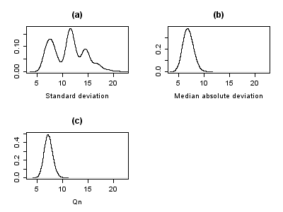 Statistics distributions obtained from Simon Newcomb speed of light dataset obtained through bootstrapping: result differs between the standard deviation and the median absolute deviation (both measures of dispersion) distributions.
This gives us ability to improvise our model for robustness by establishing rules for unstable conditions within the data. It is to be noted that while bootstrapping there exists at-least a very smaller subset of data that corresponds to all the clusters within the larger dataset.Bootstrapping allows assigning measures of accuracy defined in terms of bias, variance, confidence intervals, prediction error.
Statistics distributions obtained from Simon Newcomb speed of light dataset obtained through bootstrapping: result differs between the standard deviation and the median absolute deviation (both measures of dispersion) distributions.
Let’s now see what’s Random Forests for Classification!

Random Forest is a classification method / technique that is based on decision trees. Unlike the traditional decision tree classification technique, random forest classifier proceeds by growing many decision trees in was that can address the model reproducibility. In the traditional decision tree classification there exists an optimal split, using which we can decide either to classify a property to be true or false, whereas, the random forest contains several such trees as a forest that will allow us to make several such binary splits in the data there by establishing complex rules for classification. These rules help us determine the predictor - target pair. In decision trees, initially all the nodes of the variable are to be searched every time while looking for an optimal split while in the random forest we split the entire data of a variable depending upon its relationship/ correlation with the target variable.The correlation is calculated by a formula known as the Gini Index.
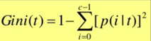 Give me a wish Mr Gini!
A Gini score gives an idea of how good a split is by how mixed the classes are in the two groups created by the split. A perfect separation results in a Gini score of 0, whereas the worst case split that results in 50/50 classes in each group results in a Gini score of 1.0. First a subset of entire data is selected at random and the best split is chosen depending upon its correlation with the target variable. Upon obtaining the best split, a random set of variables is selected from the subset that falls in the true portion of the split point. This process is continued until there is a termination/ leaf that contains ideally a single observation of a variable. The process of growing of trees in the random forest is not only dependent upon the split points obtained subsequently but also is a result of the random subsets chosen from the originally large data.This process of randomly selecting the observations of different variables is called bagging as explained before. The percentage data that is randomly selected generally varies depending upon the type of data, other parameters. The model is tested for its robustness by providing a new set of data and predict the outcomes.
There’s always mathematics to rescue!
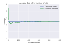
The other two things that I wish to share are the Law of Large Numbers and Central Limit theorem, in Random Forests context. Law of large numbers is an essential theorem in probability theory as well as practises that, a greater number of times a given experiment is performed, the average of the results thus obtained is close to expected value. Given, an experiment is random, the more the number of trials of experiment, closer is the average of the outcomes of all the experiments to that of the expected value.</p>
 Average
From LLN, a short form for Law of Large Numbers, it can be implied that
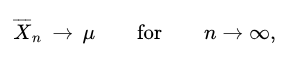 Law of Large Numbers
Law of Large Numbers Baby!where n is the number of attempts of conducting the experiment. Just opposite to the LNN is the WLN - The weak law of numbers which tells us that lesser the amount of data the mean/ average of results of the experiment tends to move closer to zero or away from 1 which is undesired.
 Limits yo!
The Central Limit Theorem!!! With origins in the Probability Theory, The Central Limit Theorem can be applied to various processes which tend to give a lot random variables.
Central Limit Theorem states that in situations where independent random variables which are normally distributed are added together, their normalized sum leads to a normal distribution which is a bell curve representing a Gaussian Distribution. It can otherwise be stated as the mixture of ‘n’ non-identical random processes in a system results in a Gaussian Process. This assumption helps us to bring in another assumption that the Law of Large Numbers holds true for such a mixture of processes and the characteristics of the process can be estimated with the help of derived parameters such as the mean. The above two assumptions also give rise to the facts that there needs to be a relatively optimum sampling rate and sampling interval for an experiment so as the subset data derived from the entire data can be used as a representative of the experiment.
With all the above text having a lot of jargon demystified, I hope reading this article has given you my insight of dealing with machine learning!
Originally posted on medium